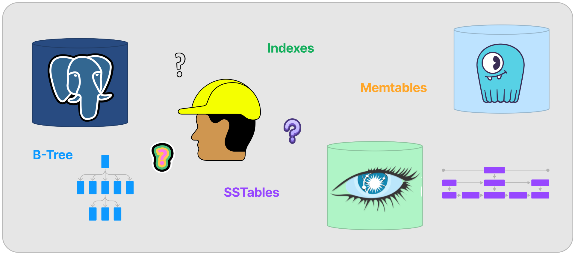
Welcome to the second installment of my blog series on the system architecture lessons from the book Designing Data-Intensive Applications by Martin Kleppman.

In this episode, we're gonna talk about database internals, such as storage, query languages, and indexes.

Let's get it.

Database Storage Approaches

Instead of diving into modern database storage systems, I love how Kleppman walks us up from the most straightforward storage and indexing structures you might try when building a toy database for some simple purpose. Seeing how they build upon each other and create new tradeoffs is fun.

Following his example, let's begin by describing a simple log-based system.

Appendable Log

When you think about storage, I'd like you to think back to the days of tape storage. It may seem ancient, but it was the preferred medium for about 30 years and is still used to this day.

The tool I used for backups more than any other in my Sysadmin days was tar, which stands for Tape ARchive.

When writing to tape, everything is linear. Think about the linked-list data structure.

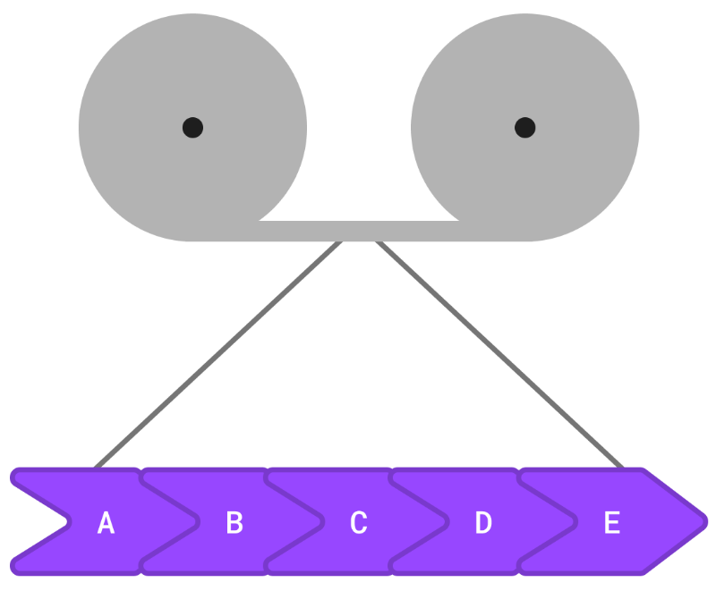
Each node contains data and a pointer to the next node (and the previous node, if they're doubly linked). Because this type of data structure was well suited to a long piece of tape, the earliest databases used a similar approach called an "appendable log."

It works by adding new rows of data to the end of a file. Each row points to the next one in the list. It is a fast way of writing data - sequential writes are still much faster than random writes on even the most cutting-edge SSDs and memory chips. Once the log file becomes too large for our filesystem, we can simply start a new one as a continuation.

The problem comes when you need to fetch that data.

You'll understand if you've ever had to use terrible tools like Notepad to view a log file. You're looking at this file, where everything is ordered from oldest at the top to newest at the bottom, but you need to find a log line that happened somewhere in the middle. If you can't search the file, then the only thing to do is start scrolling. You read date after date until you finally see the one you want. Then you scroll some more until you see the hour, and more for the minute, and finally the second and millisecond.

This process is what a database must do when fetching records from a linear appendable log. Just keep hopping from one record to the next in linear time until it finds the key.

Rows of data being searched on at a time

"Why don't we just sort it?" you might ask. That's very clever. You get a gold star! ⭐️

Sorting is a significant improvement. We can find things much faster than before by using a binary search algorithm on our sorted log. In O(log n) time, in fact. Unfortunately, this also slows down our inserts. We have to sort each key into place after every insertion. These inserts may take a logarithmic amount of time. Our unordered log file, by contrast, could handle inserts instantly. It also means every write could result in log^n^ writes as it bubbles up to the correct position in our file.

Put simply, use an unordered log if you're using a flat-file, appendable log data storage structure and need to optimize for write-heavy operations. If reads are more important, use a sorted log file. We'll dig into specific implementations of these concepts in just a minute.

If you know your Data Structures, you might now suggest a data structure with both fast insertion and retrieval time, the Hashmap!

Enter the Hashmap

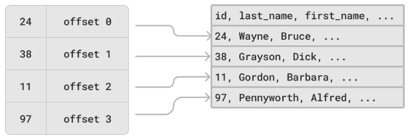
The next improvement we can try is to create a unique key for each record (whether visible to users or not) and store the location in the log where the record begins. This way, we can jump straight to that record when needed. If there are many log segments to choose from, the index can also store those pointers.

A couple of points to note about our new log + hashmap marriage:

We'll need to regularly remove duplicate records when we update or replace a record with an existing key
Logs will eventually get too big for our filesystem (or too unwieldy), so we'll need to segment them, adding complexity to our retrieval operations
The hashmap index must fit in memory and will disappear when the system restarts
Searching for a range of values still requires a linear-time search

This is where B-trees can come in handy.

B-Trees

B-Tree is the most common database indexing structure, found in two of the most popular databases, PostgreSQL and MySQL (when using InnoDB). It has a complexity of O(log n) for both inserts and retrievals.

How it works is very similar to a Binary Search Tree, or BST, but each node may contain several values. The implementation uses fixed-size pages of keys that each reference child pages with increasingly specific ranges at each level.

Additionally, the keys can be abbreviated to save space.

In a very simplistic example with a string-based index, you could have the letters A, G, L, Q, U at the head node, and each node at the next level would be the parent node character plus a few characters in the alphabet, e.g., A, B, C, D, E, F, and the level after that (again following A) might be Aa, Ag, Al, Aq, Au - very similar to the indexes you'd see in the corner of each page of a dictionary.

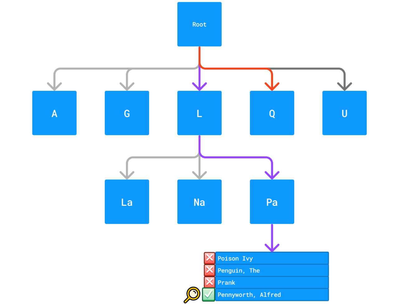
(Note that keys are not guaranteed to be sorted within any range or "page" of data).

Since inserting into any sorted tree structure requires some extra work while finding the correct position, there's a greater possibility that a crash could result in data loss. Concurrently writing data to a Write-Ahead Log (WAL) can assist with crash recovery; once the system recovers, traverse the log in reverse until the last successfully written record is found and insert everything in the WAL after that point.

Since you know your data structures, you'll note that tree insertions like this have a worst-case time of O(log n) for inserts. On the plus side, they're also O(log n) on the retrieval side. For this reason, we can say that B-Trees are read-optimized.

Some more considerations:

B-Trees require a lot of writes as they sort things into place and sometimes require rebalancing jobs to run in the background
They can be fragmented on the storage device
They can consume more space than other storage structures

Let's look at Log-Structured Merge Trees as an alternative.

Log-Structured Merge (LSM) Trees

Log-Structured Merge Trees were proposed as an alternative to B-Trees in the late '90s to allow for more performant disk write usage.

In a nutshell, an LSM-tree is comprised of two components:

In-memory index tree (often called the memtable)
On-disk appendable log(s)

Though stored as a contiguous log, the structure maintains node IDs and references to support tree traversals similar to a B-Tree (or exactly that, in some cases). In contrast to B-Trees, data is not overwritten when a key is updated. New data is appended, and the more recent values are returned on fetch. This structure has the additional advantage of sequential writes, a valuable optimization we saw earlier when comparing sorted and unsorted log files. Deleted and outdated data are marked with a tombstone attribute to indicate they are no longer valid.

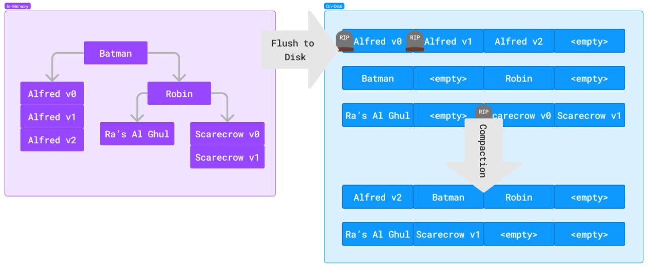
A typical write will be first written to the write ahead log (WAL), followed by an index write to the memtable. Once the memtable starts nearing capacity, a background job will begin flushing indexes to disk.

Another background job will periodically compact the log, removing outdated copies of duplicated keys.

10-years after LSM-trees were proposed, one of the most popular implementations, Sorted String Tables (SSTables), was created at Google for their BigTable database.

Sorted-String Tables (SSTables) 🐍

SSTables are a storage system used by Apache Cassandra and ScyllaDB. The structure builds upon LSM-Trees by ensuring the keys and indexes are sorted.

The ScyllaDB and Cassandra implementations use a skip-list data structure as the memtable, which records all writes and serves as many reads as possible. Writes to the commit log occur in tandem. Once the memtable nears a configured limit, it flushes to disk.

When a flush occurs, the memtable is written to disk as a Sorted String Table. This structure is similar to our original appendable, segmented log structure, except that sorted string-based keys index each record. We can also keep a sparse index in memory for even faster retrieval.

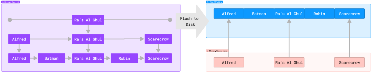
Illustration of SSTables memtable, sorted-string log, and sparse index

Sorted keys enable us to jump to the nearest key and scan from there, even when using a sparse in-memory index. This structure also has the advantage of making range queries much faster, unlike our previous models. If that isn't enough to sell you, it can also aid with full-text and fuzzy finding. Think about it: all lexicographically similar keys will be near each other. Easy!

In the case of Cassandra, these SSTables are read-only. Updates are handled by creating duplicate records with a newer timestamp. Deletes are handled by creating a 'tombstone' marker for each record to be destroyed.

Periodically, these SSTables are merged and compacted. A new SSTable is created by performing a similar operation to merge-sort. During this process, tombstone-referenced records and duplicated keys with older timestamps are excluded from the new SSTable. (Ref)

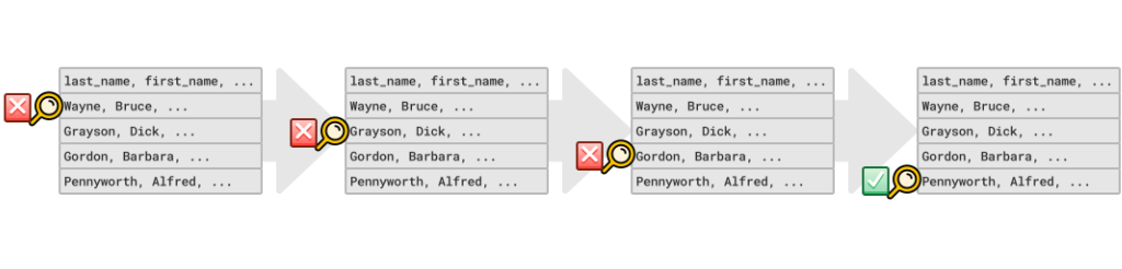
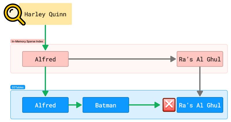
This structure is great for range queries, and specific keys can be found in O (log n) time, but what happens if a key is not found?

In this case, our search would pass through the memtable, pick a point between two indexes on disk, and do a disk scan only to return empty-handed.

Illustration of a search failing to find a record on an SSTable, requiring linear time search

How can we avoid all the work for data that doesn't even exist? For that, many look to bloom filters.

Bloom Filters 🌻

In case you haven't encountered them yet, Bloom filters are a space and time-efficient data structure for discovering the non-existence of an item.

How it works:

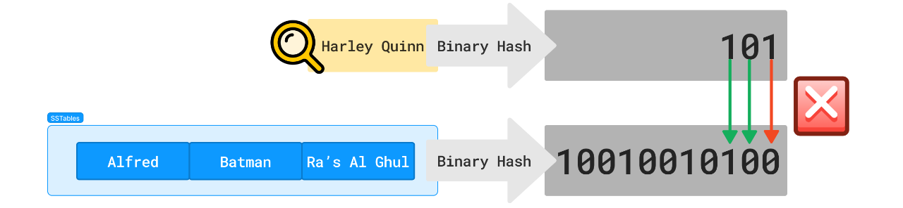
First, you initialize a binary array of all zeros as your filter
A hash function converts each of your keys to a binary hash
Each key is stored in the original string by flipping the corresponding bits to '1'
When looking up a given string, the hash function returns the key
Compare the hash to the filter
If any of the bits in our hash are zero in the filter, the key does not exist
If all the bits are matched, then maybe it exists. Time to scan!

The space for a bloom filter is relatively small. You could store 1 million keys sized 1KB each with a false-positive rate close to 1 in a million in about 3.35GB. Increasing the false-positive probability to 1 in ~10M only raises it to 3.9GB.

Time-wise, the lookup occurs in O(1) constant time. 🏎💨

Illustration of a bloom filter indicating that a key doesn't exist

So there still isn't a better way to find out if a key exists; only a unique index can tell with certainty if a key exists, but at least we can find out quickly if a key doesn't exist, saving us a lot of unnecessary disk accesses.

Summary

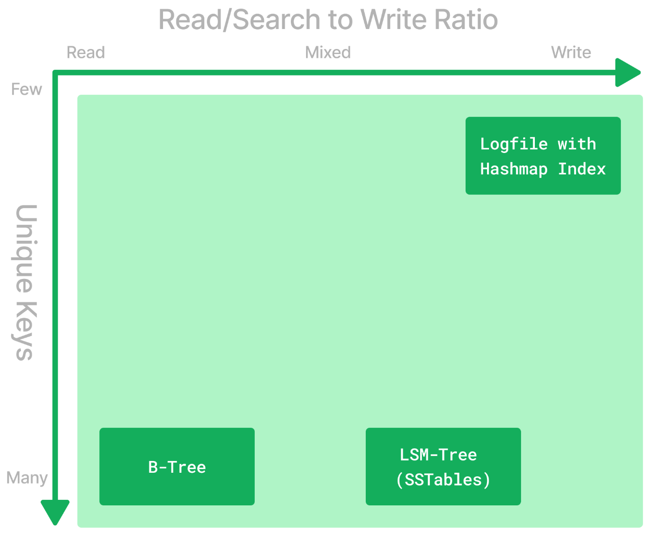
There are a few tradeoffs to consider when picking a database according to how it stores and indexes data. Here's how we might use what we learned here to make an educated guess on the best engine for our use-case:

Case 1: Write-heavy workload. Searching isn't needed:
- Use a simple log and keep appending to it.
Case 2: Write-heavy workload. Searching must be fast. Number of unique keys is small.
- Use a simple log with a Hash Table Index
Case 3: Read-heavy workload. Searching must be fast. Number of unique keys is large.
- B-Trees are the most popular choice!
Case 4: Write-heavy or mixed workload. Searching must be fast. Number of unique keys is large.
- LSM-Trees with SSTables and Bloom Filters will get you far!

Grid with read write ratio on one axis and unique keys on another showing where each storage option falls

Not covered in DDIA are vector databases, which are quickly gaining popularity right now due to their usage with LLMs. I'll link back here when I've got a similar rundown on those.

Keep an eye out for our next episode, where we'll dig into encoding data for transmission.

If you like what you read or want to continue the conversation, I'd love to hear from you: nate@natecornell.com.

Data Storage and Indexing